3 Motivating data
This paper focuses on a type of psychometric experiment called a temporal order judgment (TOJ) experiment. If there are two distinct stimuli occurring nearly simultaneously then our brains will bind them into a single percept (perceive them as happening simultaneously). Compensation for small temporal differences is beneficial for coherent multisensory experiences, particularly in visual-speech synthesis as it is necessary to maintain an accurate representation of the sources of multisensory events.
It was Charles Darwin who in his book “On the Origin of Species” developed the idea that living organisms adapt in order to better survive in their environment. Sir Francis Galton, inspired by Darwin’s ideas, became interested in the differences in human beings and in how to measure those differences. Galton’s works on studying and measuring human differences lead to the creation of psychometrics – the science of measuring mental faculties. Around the same time that he was developing his theories, Johann Friedrich Herbart was also interested in studying consciousness through the scientific method, and is responsible for creating mathematical models of the mind.
E.H. Weber built upon Herbart’s work, and sought out to prove the idea of a psychological threshold. A psychological threshold is a minimum stimulus intensity necessary to activate a sensory system – a liminal stimulus. He paved the way for experimental psychology and is the namesake of Weber’s Law (Equation (3.1)), which states that the change in a stimulus that will be just noticeable is a constant ratio of the original stimulus (Ekman 1959).
\[\begin{equation} \frac{\Delta I}{I} = k \tag{3.1} \end{equation}\]
To demonstrate this law, consider holding a 1 kg weight (\(I = 1\)), and further suppose that the difference between a 1 kg weight and a 1.2 kg weight (\(\Delta I = 0.2\)) can just be detected. Then the constant just noticeable ratio is:
\[k = \frac{0.2}{1} = 0.2\]
Now consider picking up a 10 kg weight. The mass required to just detect a difference can be calculated as:
\[\frac{\Delta I}{10} = 0.2 \Rightarrow \Delta I = 2\]
The difference between a 10 kg and a 12 kg weight is expected to be just barely perceptible. Note that the difference in the first set of weights is 0.2, and in the second set it is 2. The perception of the difference in stimulus intensities is not absolute, but relative. G.T. Fechner devised the law (Weber-Fechner Law, Equation (3.2)) that the strength of a sensation grows as the logarithm of the stimulus intensity.
\[\begin{equation} S = K \ln I \tag{3.2} \end{equation}\]
Consider two light sources: one that is 100 lumens (\(S_1 = K \ln 100\)) and another that is 200 lumens (\(S_2 = K \ln 200\)). The intensity of the second light is not perceived as twice as bright, but only about 1.15 times as bright according to (3.2):
\[\theta = S_2 / S_1 \approx 1.15\]
Notice that the value \(K\) cancels out when calculating the relative intensity, but knowing \(K\) can lead to important psychological insights about differences between persons or groups of people. What biological and contextual factors affect how people perceive different stimuli? How do we measure their perception in a meaningful way? We can collect data from psychometric experiments, fit a model to the data from a family of functions called psychometric functions, and inspect key operating characteristics of those functions.
3.1 Psychometric experiments
Psychometric experiments are devised in a way to examine psychophysical processes, or the response between the world around us and our inward perceptions. A psychometric function relates an observer’s performance to an independent variable, usually some physical quantity of a stimulus in a psychophysical task (Wichmann and Hill 2001a). Psychometric functions were studied as early as the late 1800’s, and Edwin Boring published a chart of the psychometric function in The American Journal of Psychology in 1917 (Boring 1917).
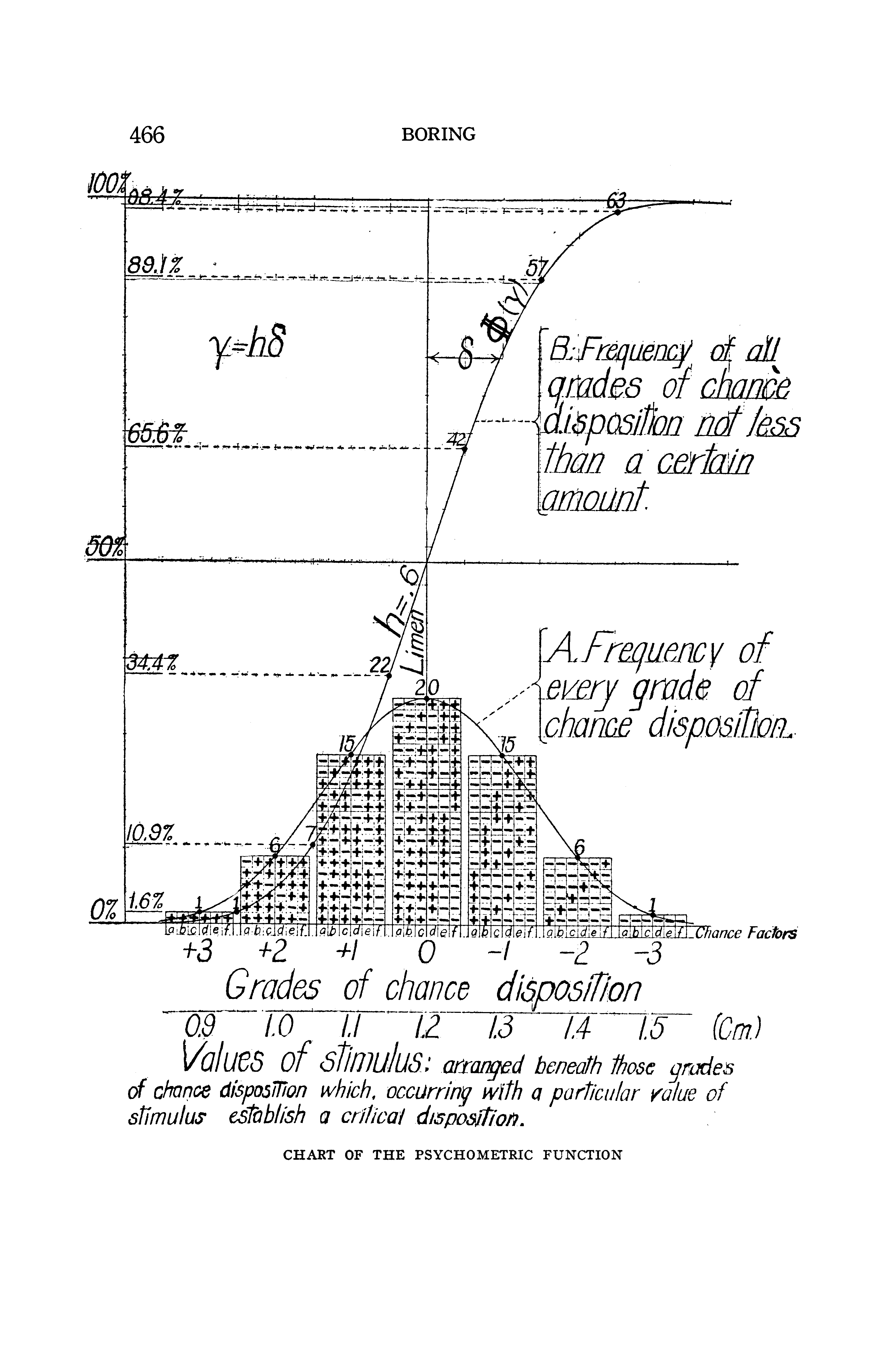
Figure 3.1: A chart of the psychometric function. The experiment in this paper places two points on a subject’s skin separated by some distance, and has them answer their impression of whether there is one point or two, recorded as either two points or not two points. As the separation of aesthesiometer points increases, so too does the subject’s confidence in their perception of two-ness. So at what separation is the impression of two points liminal?
Figure 3.1 displays the key aspects of the psychometric function. The most crucial part is the sigmoid function, the S-like non-decreasing curve which in this case is represented by the Normal CDF, \(\Phi(\gamma)\). The horizontal axis represents the stimulus intensity: the separation of two points in centimeters. The vertical axis represents the probability that a subject has the impression of two points. With only experimental data, the response proportion becomes an approximation for the probability.
The temporal asynchrony between stimuli is called the stimulus onset asynchrony (SOA), and the range of SOAs for which sensory signals are integrated into a global percept is called the temporal binding window. When the SOA grows large enough, the brain segregates the two signals and the temporal order can be determined.
Our experiences in life as we age shape the mechanisms of processing multisensory signals, and some multisensory signals are integrated much more readily than others. Perceptual synchrony has been previously studied through the point of subjective simultaneity (PSS) – the temporal delay between two signals at which an observer is unsure about their temporal order (Stone et al. 2001). The temporal binding window is the time span over which sensory signals arising from different modalities appear integrated into a global percept.
A deficit in temporal sensitivity may lead to a widening of the temporal binding window and reduce the ability to segregate unrelated sensory signals. In TOJ tasks, the ability to discriminate the timing of multiple sensory signals is referred to as temporal sensitivity, and is studied through the measurement of the just noticeable difference (JND) – the smallest lapse in time so that a temporal order can just be determined.
Figure 3.2 highlights the features through which we study psychometric functions. The PSS is defined as the point where an observer can do no better at determining temporal order than random guessing (i.e. when the response probability is 50%). The JND is defined as the extra temporal delay between stimuli so that the temporal order is just able to be determined. Historically this has been defined as the difference between the 84% level – one standard deviation away from the mean – and the PSS, though the upper level often depends on domain expertise.
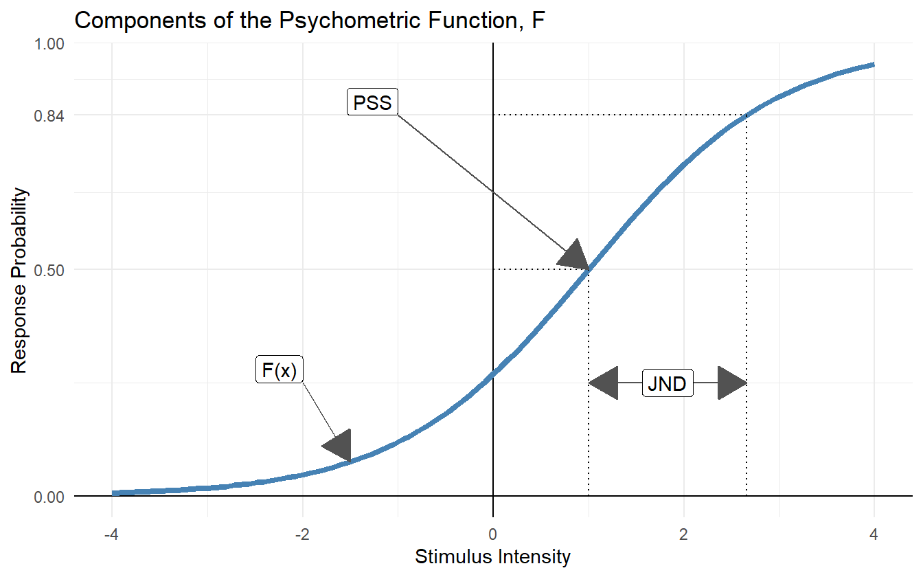
Figure 3.2: The PSS is defined as the point where an observer can do no better at determining temporal order than random guessing. The just noticeable difference is defined as the extra temporal delay between stimuli so that the temporal order is just able to be determined. Historically this has been defined as the difference between the 0.84 level and the PSS, though the upper level depends on domain expertise.
3.2 Temporal order judgment tasks
The data set used in this paper comes from small-scale preliminary experiments done by A.N. Scurry and Dr. Jiang in the Department of Psychology at the University of Nevada. Reduced temporal sensitivity in the aging population manifests in an impaired ability to perceive synchronous events as simultaneous, and similarly more difficulty in segregating asynchronous sensory signals that belong to different sources. The consequences of a widening of the temporal binding window is considered in Scurry et al. (2019), as well as a complete detailing of the experimental setup and recording process. Here we present a shortened summary of the experimental methods.
There are four different tasks in the experiment: audio-visual, visual-visual, visual-motor, and duration, and each task is respectively referred to as audiovisual, visual, sensorimotor, and duration. The participants consist of 15 young adults (age 20-27), 15 middle age adults (age 39-50), and 15 older adults (age 65-75), all recruited from the University of Nevada, Reno. Additionally all subjects are right handed and are reported to have normal or corrected to normal hearing and vision.
| soa | response | sid | task | block | age_group | age | sex |
|---|---|---|---|---|---|---|---|
| -350 | 0 | O-m-BC | audiovisual | baseline | older | 70 | M |
| 200 | 1 | M-f-TW | visual | adapt1 | middle | 49 | F |
| 28 | 1 | O-f-KK | sensorimotor | baseline | older | 66 | F |
| 150 | 1 | Y-m-CB | duration | adapt1 | young | 22 | M |
In the audiovisual TOJ task, participants were asked to determine the temporal order between an auditory and visual stimulus. Stimulus onset asynchrony values were selected uniformly between -500 to +500 ms with 50 ms steps, where negative SOAs indicated that the visual stimulus was leading, and positive values indicated that the auditory stimulus was leading. Each SOA value was presented 5 times in random order in the initial block. At the end of each trial the subject was asked to report if the auditory stimulus came before the visual, where a \(1\) indicates that they perceived the sound first, and a \(0\) indicates that they perceived the visual stimulus first.
A similar setup is repeated for the visual, sensorimotor, and duration tasks. The visual task presented two visual stimuli on the left and right side of a display with temporal asynchronies that varied between -300 ms to +300 ms with 25 ms steps. Negative SOAs indicated that the left stimulus was first, and positive that the right came first. A positive response indicates that the subject perceived the right stimulus first.
The sensorimotor task has subjects focus on a black cross on a screen. When it disappears, they respond by pressing a button. Additionally, when the cross disappears, a visual stimulus was flashed on the screen, and subjects were asked if they perceived the visual stimulus before or after their button press. The latency of the visual stimulus was partially determined by individual subject’s average response time, so SOA values are not fixed between subjects and trials. A positive response indicates that the visual stimulus was perceived after the button press.
The duration task presents two vertically stacked circles on a screen with one appearing right after the other. The top stimulus appeared for a fixed amount of time of 300 ms, and the bottom was displayed for anywhere between +100 ms to +500 ms in 50 ms steps corresponding to SOA values between -200 ms to +200 ms. The subject then responds to if they perceived the bottom circle as appearing longer than the top circle.
| Task | Positive Response | Positive SOA Truth |
|---|---|---|
| Audiovisual | Perceived audio first | Audio came before visual |
| Visual | Perceived right first | Right came before left |
| Sensorimotor | Perceived visual first | Visual came before tactile |
| Duration | Perceived bottom as longer | Bottom lasted longer than top |
Perceptual synchrony and temporal sensitivity can be modified through a baseline understanding. In order to perceive physical events as simultaneous, our brains must adjust for differences in temporal delays of transmission of both psychical signals and sensory processing (Fujisaki et al. 2004). In some cases such as with audiovisual stimuli, the perception of simultaneity can be modified by repeatedly presenting the audiovisual stimuli at fixed time separations (called an adapter stimulus) to an observer (Vroomen et al. 2004). This repetition of presenting the adapter stimulus is called temporal recalibration.
After the first block of each task was completed, the participants went through an adaptation period where they were presented with the respective stimuli from each task repeatedly at fixed temporal delays, then the TOJ task was repeated. To ensure that the adaptation affect persisted, the subject was presented with the adapter stimulus at regular intervals throughout the second block. The blocks are designated as pre and post1, post2, etc. in the data set. In this paper we only focus on the baseline block (pre) and the post-adaptation block (post1).
3.3 Data visualization and quirks
The dependent variable in these TOJ experiments is the subject’s perceived response, encoded as a 0 or a 1, and the independent variable is the SOA value. If the response is plotted against the SOA values, then it is difficult to determine the relationship (see the right panel of figure 3.3). Transparency can be used to better visualize the relationship. The center panel in figure 3.3 shows the same data as the left, except that the transparency is set to \(0.05\). Note that there is a higher density of “0” responses towards more negative SOAs, and a higher density of “1” responses for more positive SOAs. The proportion of “positive” responses for a given SOA is computed and plotted against the SOA value (displayed in the right panel of figure 3.3). The relationship between SOA values and responses is clear – as the SOA value goes from more negative to more positive, the proportion of positive responses increases from near 0 to near 1.
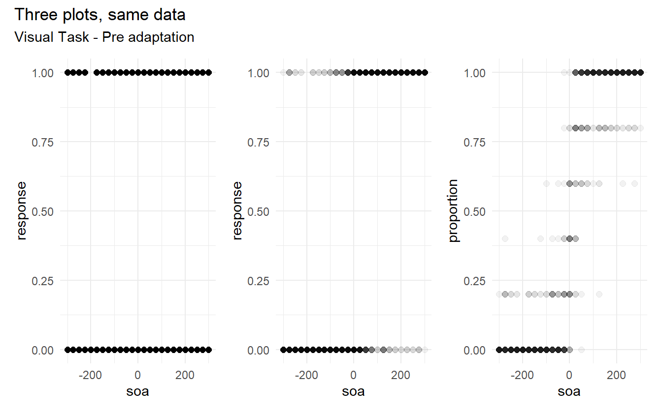
Figure 3.3: Left: Simple plot of response vs. soa value. Center: A plot of response vs. soa with transparency. Right: A plot of proportions vs. soa with transparency.
The right panel in figure 3.3 is the easiest to interpret, and we often present the observed and predicted data using the proportion of responses rather than the raw responses. Proportional data is also bounded on the same interval as the response in contrast to the raw counts.
For the audiovisual task, the responses can be aggregated into binomial data – the number of positive responses for given SOA value – which is more efficient to work with than the Bernoulli data (see table 3.5). However the number of times an SOA is presented varies between the pre-adaptation and post-adaptation blocks; 5 and 3 times per SOA respectively.
| block | soa | n | k | proportion |
|---|---|---|---|---|
| baseline | 200 | 5 | 4 | 0.80 |
| 150 | 5 | 5 | 1.00 | |
| -350 | 5 | 0 | 0.00 | |
| adapt1 | 350 | 3 | 3 | 1.00 |
| -500 | 3 | 1 | 0.33 | |
| -200 | 3 | 0 | 0.00 |
There is one younger subject that did not complete the audiovisual task, and one younger subject that did not complete the duration task. There is also one older subject who’s response data for the post-adaptation audiovisual task is unreasonable – it is extremely unlikely that the data represents genuine responses (see figure 3.4).
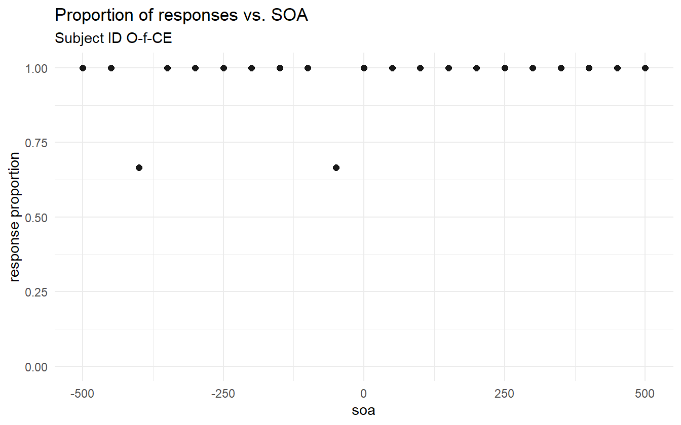
Figure 3.4: Post-adaptation response data for O-f-CE
Of all the negative SOAs, there were only two “correct” responses (the perceived order matches the actual order). If a subject is randomly guessing the temporal order, then a naive estimate for the proportion of correct responses is 0.5. If a subject’s proportion of correct responses is above 0.5, then they are doing better than random guessing. Figure 3.5 shows that subject O-f-CE is the only one who’s proportion is below 0.5 (and by a considerable amount), and so their post-adaptation block is removed from data set for model fitting.
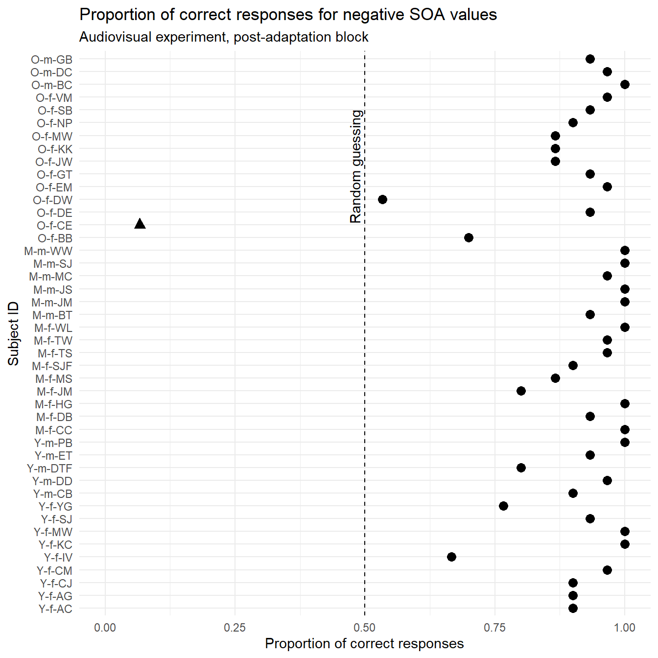
Figure 3.5: Proportion of correct responses for negative SOA values during the post-adaptation audiovisual experiment.