5 Psychometric Results
What was the point of going through all the work of building a model if not to answer the questions that motivated the model in the first place? To reiterate, the questions pertain to how the brain reconciles stimuli originating from different sources, and if biological (age) and contextual (task, temporal recalibration) factors contribute to global percepts. The way through which these questions are answered is through a psychometric experiment and the resulting psychometric function (chapter 3). This chapter is divided into three sections: the affects of temporal recalibration on perceptual synchrony, the affects of temporal recalibration on temporal sensitivity, and the consideration of a lapse rate. Also recall that there are four separate tasks - audiovisual, visual, duration, and sensorimotor.
Temporal recalibration consists of presenting a subject with an adapting stimulus throughout a block of a psychometric experiment. Depending on the mechanisms at work, the resulting psychometric function can either be shifted (biased) towards the adapting stimulus (lag adaption) or away (Bayesian adaptation). The theory of integrating sensory signals is beyond the scope of this paper, but some papers discussing sensory adaptation in more detail are Miyazaki et al. (2006), Sato and Aihara (2011), and Stocker and Simoncelli (2005). The statistical associations are reported without consideration for the deeper psychological theory.
5.1 On Perceptual Synchrony
Perceptual synchrony is when the temporal delay between two stimuli is small enough so that the brain integrates the two signals into a global percept - perceived as happening simultaneously. Perceptual synchrony is studied through the point of subjective simultaneity (PSS), and in a simple sense represents the bias towards a given stimulus. Ideally the bias would be zero, but human perception is liable to change due to every day experiences. The pre-adaptation block is a proxy for implicit bias, and the post-adaptation indicates whether lag or Bayesian adaptation is taking place. Some researchers believe that both forms of adaptation are taking place at all times and that the mixture rates are determined by biological and contextual factors. We try to stay away from making any strong determinations and will only present the results conditional on the model and the data.
Audiovisual TOJ Task
There are two ways that we can visually draw inferences across the six different age-block combinations. The distributions can either be faceted by age group, or they can be faceted by block. There are actually many ways that the data can be presented, but these two methods of juxtaposition help to answer two questions - how does the effect of adaptation vary by age group, and is there a difference in age groups by block? The left hand plot of figure 5.1 answers the former, and the right hand plot answers the latter.
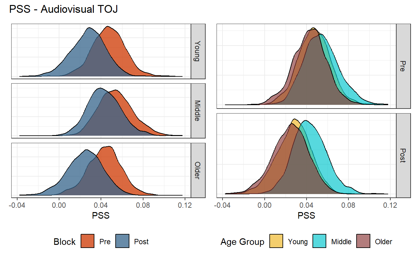
Figure 5.1: Posterior distribution of PSS values for the audiovisual task.
Across all age groups, temporal recalibration results in a negative shift towards zero in the PSS (as shown by the left hand plot), but there is no significant difference in the PSS between age groups (right hand plot). A very convenient consequence of using MCMC is that the samples from the posterior can be recombined in many ways to describe new phenomena. The PSS values can even be pooled across age groups so that the marginal affect of recalibration may be considered (left hand plot of figure 5.2).
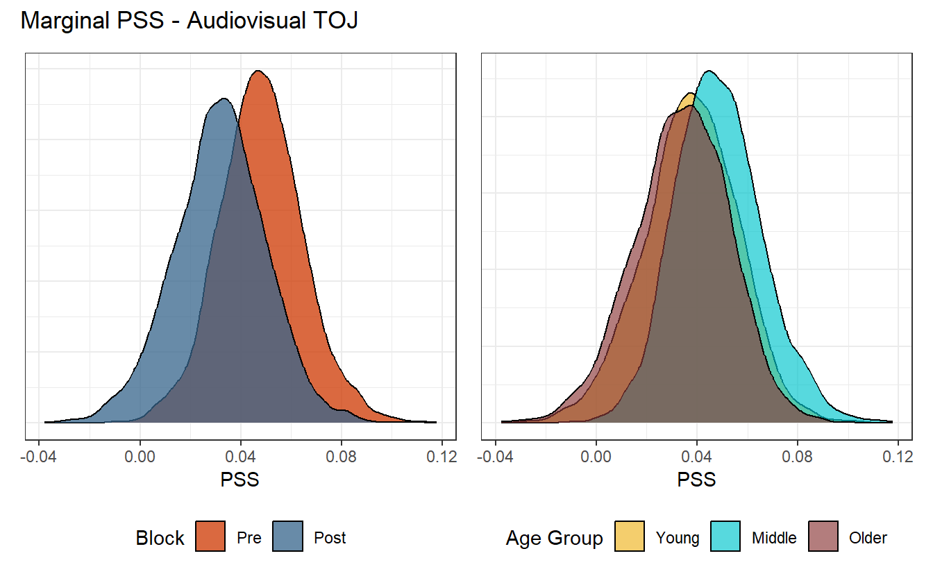
Figure 5.2: Posterior distribution of PSS values for the audiovisual task. Left: Marginal over age group. Right: Marginal over block.
Now with the marginal of age group, the distribution of differences between pre- and post-adaptation blocks can be calculated. We could report a simple credible interval, but it almost seems disingenuous given that the entire distribution is available. We could report that the \(90\%\) highest posterior density interval (HPDI) of the difference is \((-0.036, 0.004)\), but consider the following figure instead (figure 5.3).
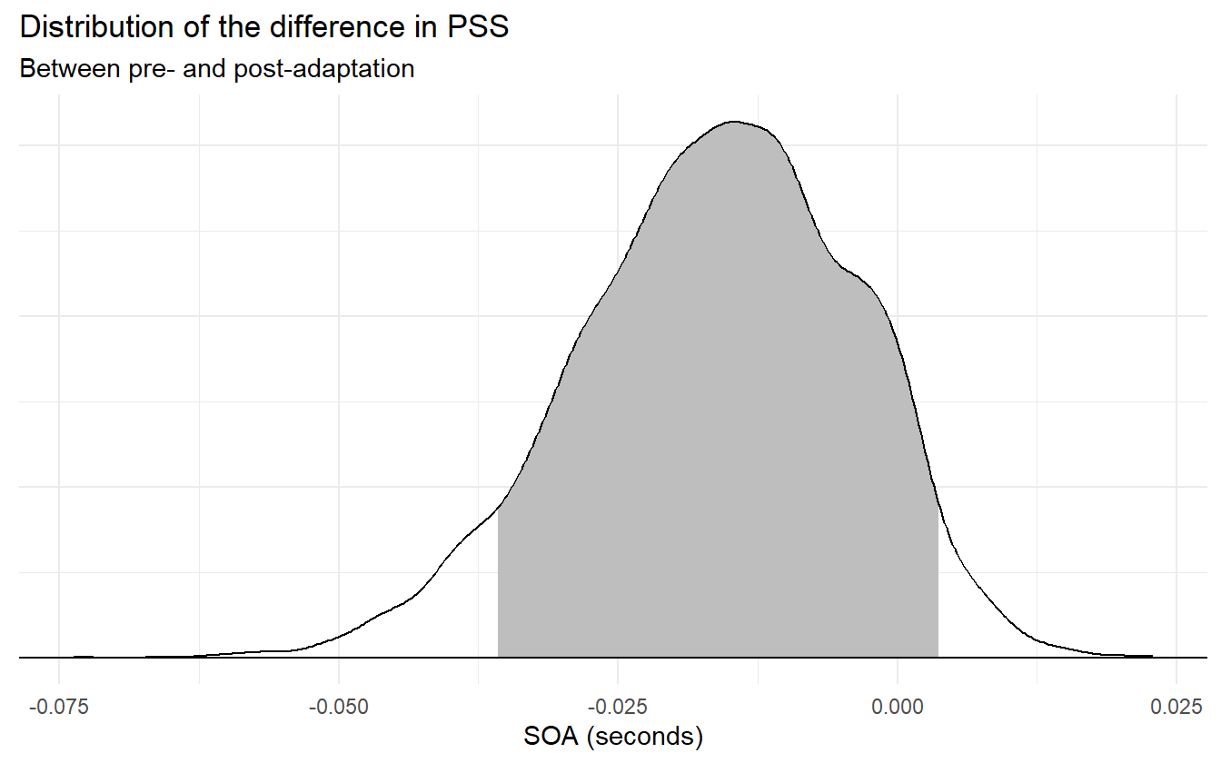
Figure 5.3: Distribution of differences for pre- and post-adaptation PSS values with 90% HPDI.
Figure 5.3 shows the distribution of differences with the \(90\%\) HPDI region shaded. From this figure, one might conclude that the effect of recalibration, while small, is still noticeable for the audiovisual task. While this could be done for every task in the rest of this chapter, it is not worth repeating as we are not trying to prove anything about the psychometric experiment itself (that is for a later paper). The point of this demonstration is simply that it can be done (and easily), and how to summarize the data both visually and quantitatively.
Visual TOJ Task
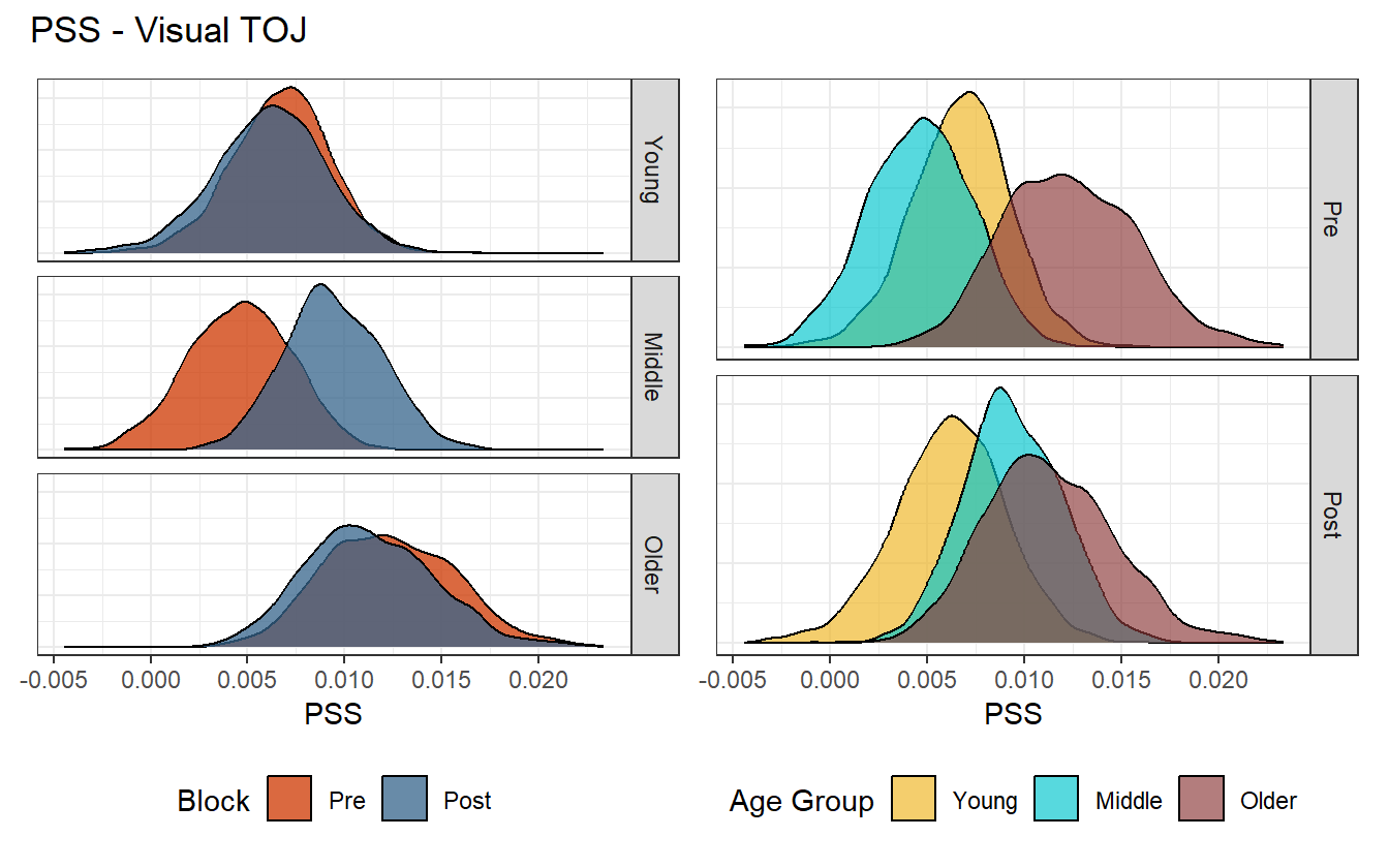
Figure 5.4: Posterior distribution of PSS values for the visual task.
Here there is no clear determination if recalibration has an effect on perceptual synchrony, as it is only the middle age group that shows a shift in bias. Even more, there is a lot of overlap between age group. Looking at the marginal distributions (figure 5.5), there may be a difference between the younger and older age groups, and the middle age and older age groups.
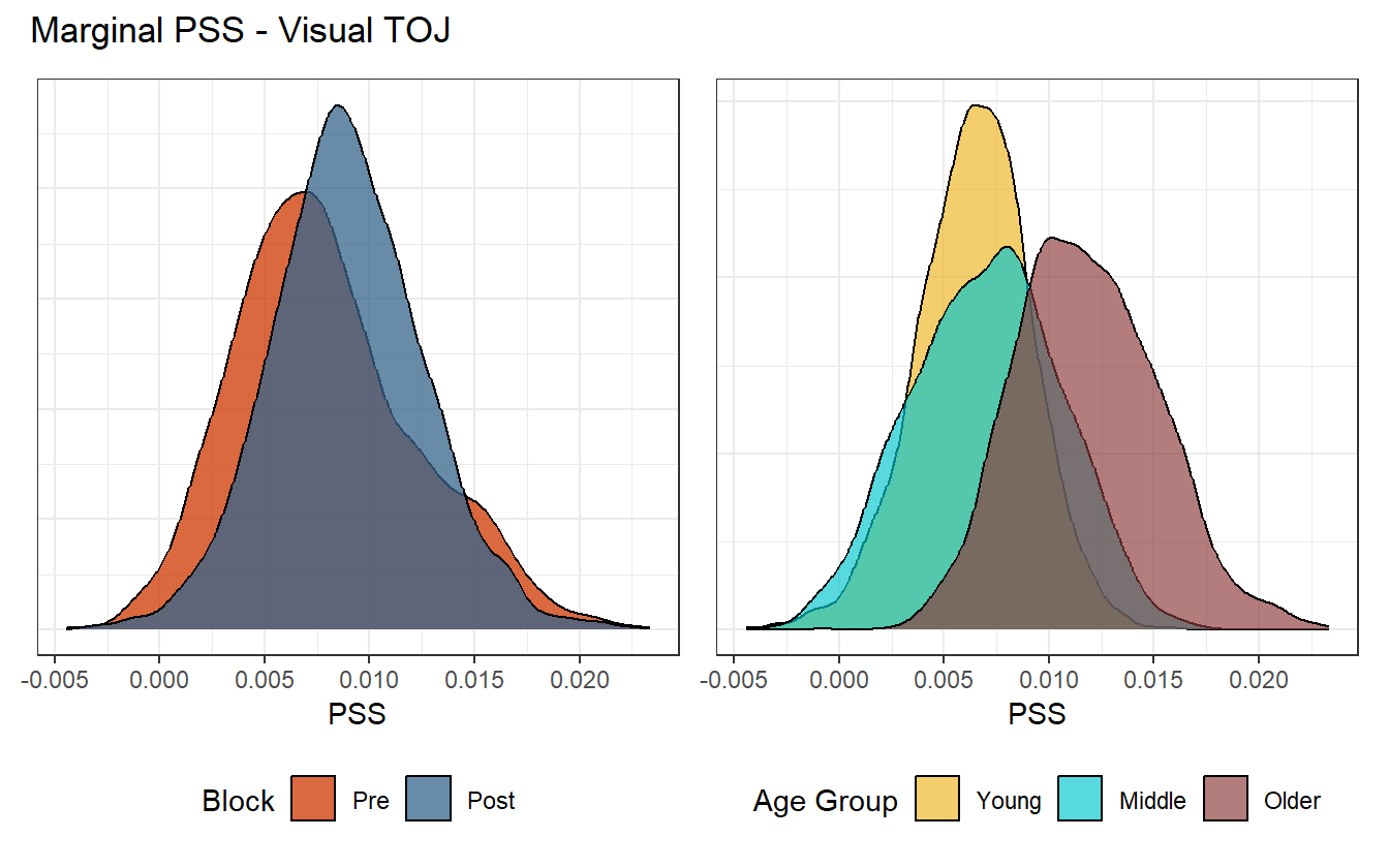
Figure 5.5: The difference between the older age group and the two others is noticeable, but not likely significant.
These plots are useful for quickly being able to determine if there is a difference in factors. If there is a suspected difference, then the distribution can be calculated from the posterior samples as needed. We suspect that there may be a difference between the older age group and the other two, so we calculate the differences and summarize them with the histogram in figure 5.6.
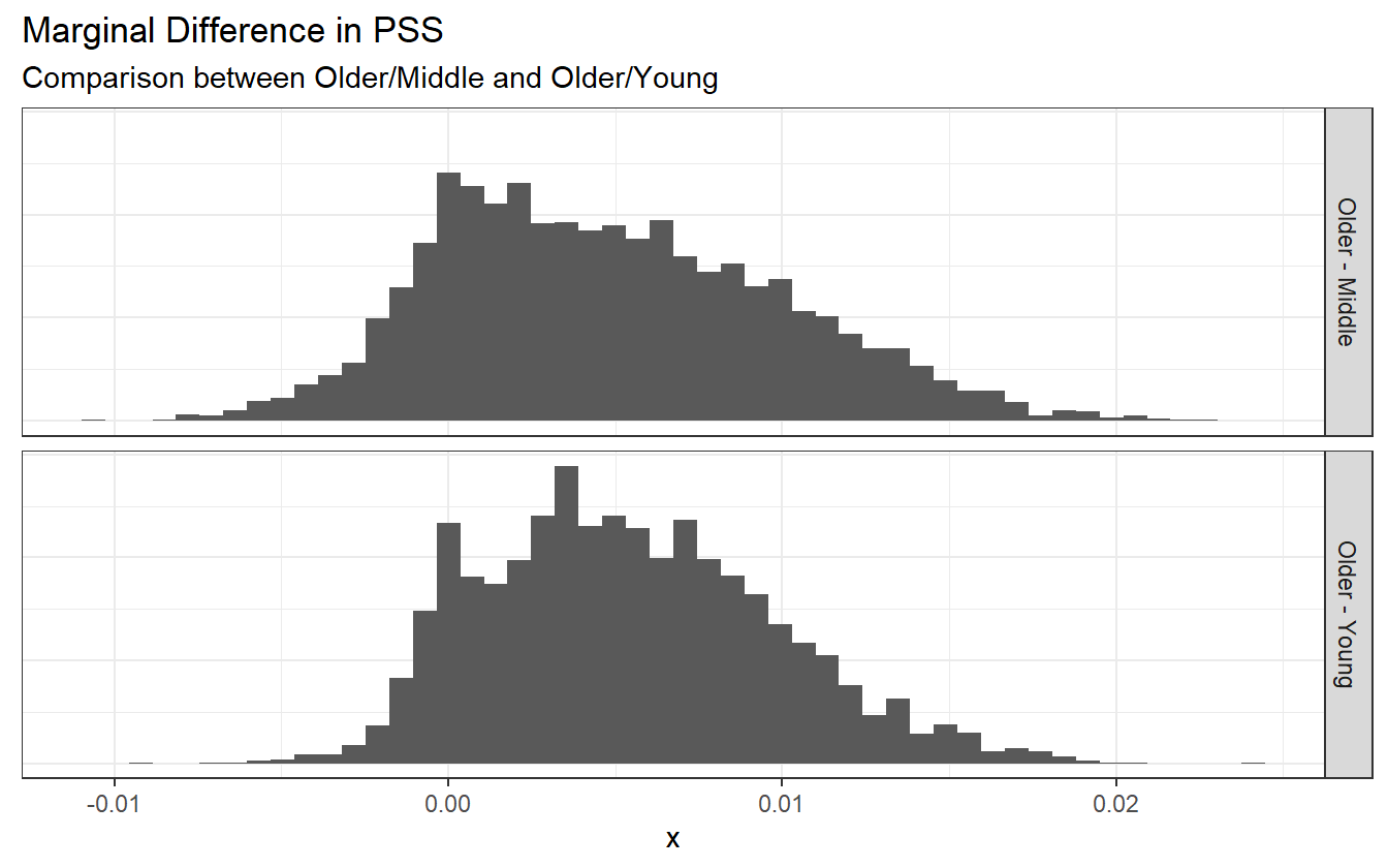
Figure 5.6: The bulk of the distribution is above zero, but there is still a chance that there is no difference in the distribution of PSS values between the age groups during the visual TOJ experiment.
The bulk of the distribution is above zero, but there is still a chance that there is no difference in the distribution of PSS values between the age groups during the visual TOJ experiment.
Duration TOJ Task
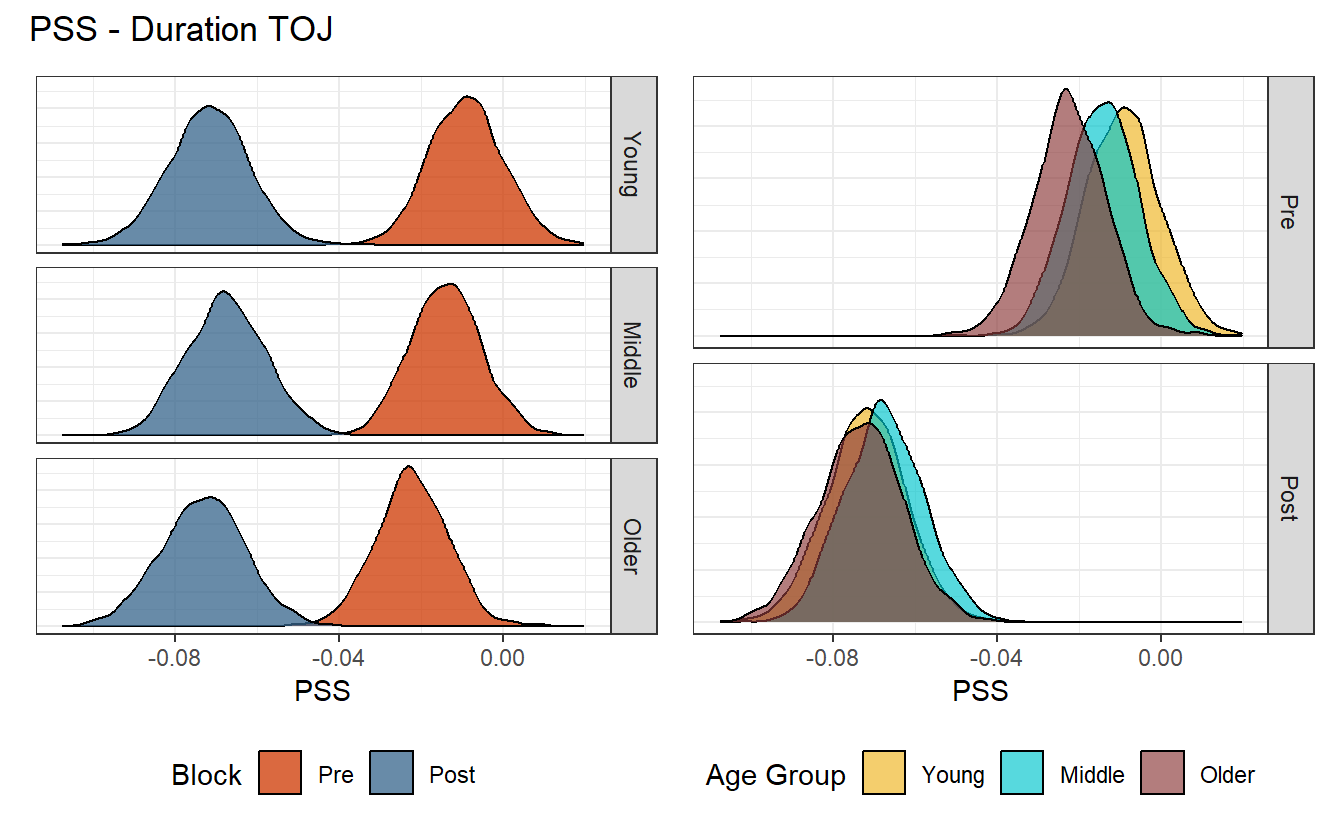
Figure 5.7: Posterior distribution of PSS values for the duration task.
The duration TOJ task is very interesting because 1) recalibration had a visually significant effect across all age groups, and 2) there is virtually no difference between the age groups. We could plot the marginal distribution, but it would not give any more insight. What we might ask is what is it about the duration task that lets temporal recalibration have such a significant effect? Is human perception of time duration more malleable than our perception to other sensory signals?
Sensorimotor TOJ Task
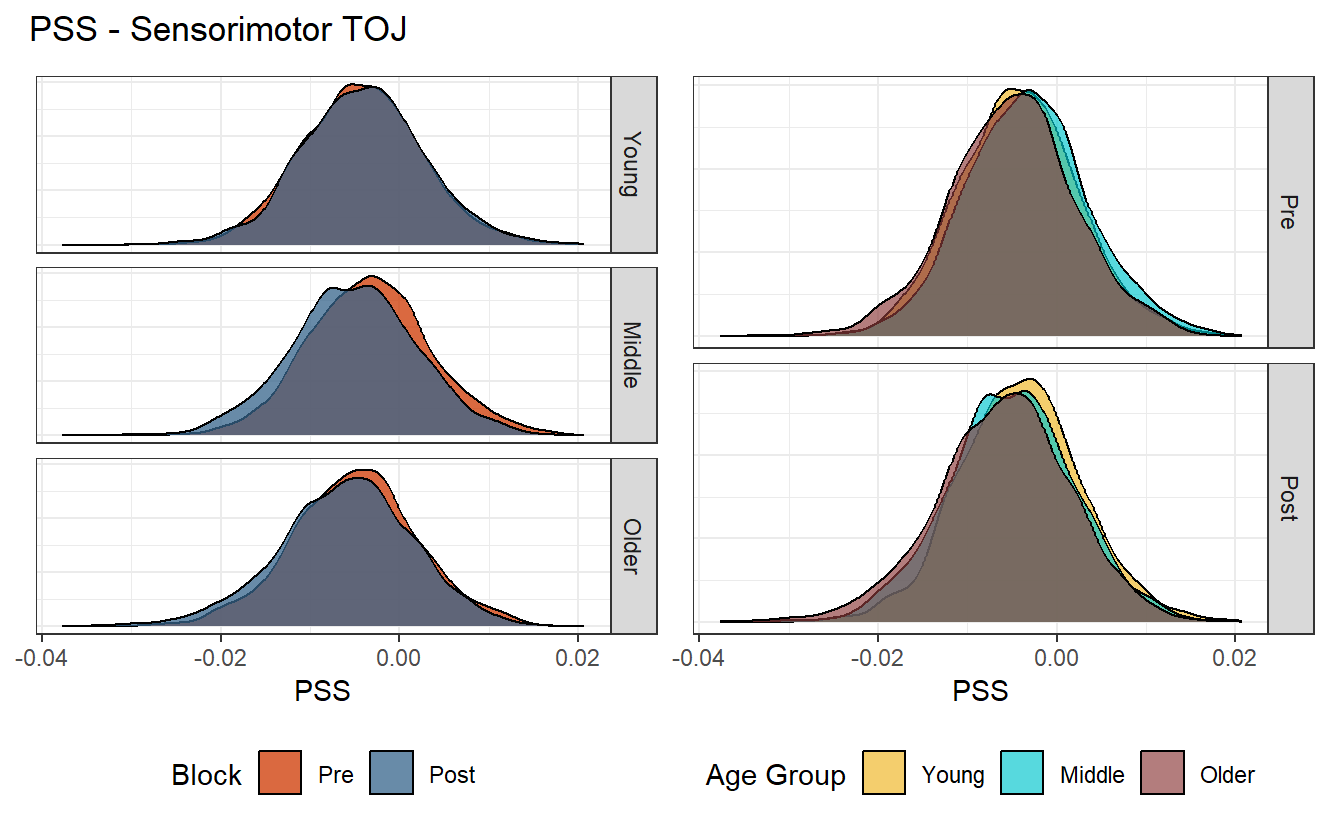
Figure 5.8: Posterior distribution of PSS values for the sensorimotor task.
There are no differences between age groups or blocks when it comes to perceptual synchrony in the sensorimotor task.
5.2 On Temporal Sensitivity
Temporal sensitivity is the ability to successfully integrate signals arising from the same event, or segregate signals from different events. When the stimulus onset asynchrony increases, the ability to bind the signals into a single percept is reduced until they are perceived as distinct events with a temporal order. Those that are more readily able to determine temporal order have a higher temporal sensitivity, and it is measured through the slope of a psychometric function - specifically the quantity known as the just noticeable difference.
Audiovisual TOJ Task
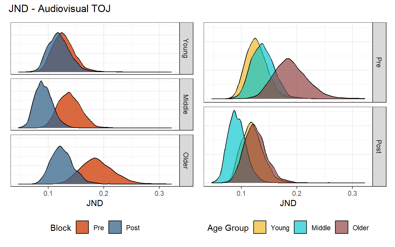
Figure 5.9: Posterior distribution of JND values for the audiovisual task.
All age groups experienced an increase in temporal sensitivity, but the effect is largest in the older age group which also had the largest pre-adaptation JND estimates. There also appears to be some distinction between the older age group and the younger ones in the pre-adaptation block, but recalibration closes the gap.
Visual TOJ Task
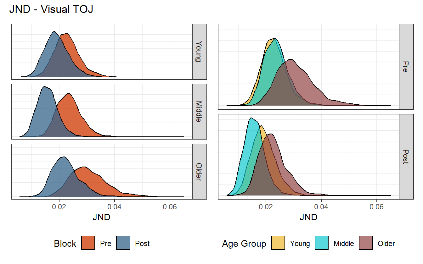
Figure 5.10: Posterior distribution of JND values for the visual task.
The story for the visual TOJ task is similar to the audiovisual one - each age group experience heightened temporal sensitivity after recalibration, with the two older age groups receiving more benefit than the younger age group. It’s also worth noting that the younger age groups have higher baseline temporal sensitivity, so there may not be as much room for improvement.
Duration TOJ Task
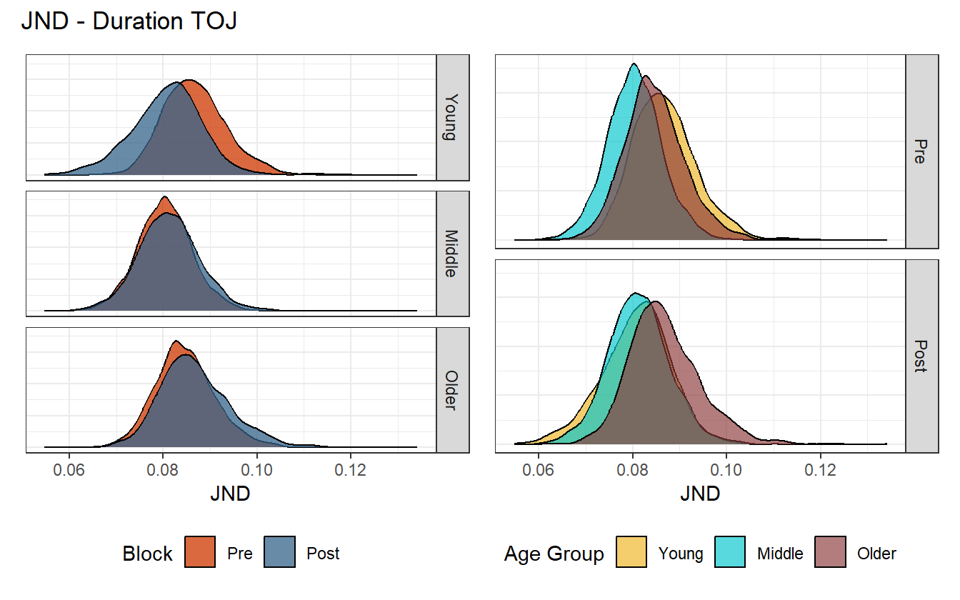
Figure 5.11: Posterior distribution of JND values for the duration task.
This time the effects of recalibration are not so strong, and just like for the PSS, there is no significant difference between age groups in the duration task.
Sensorimotor TOJ Task
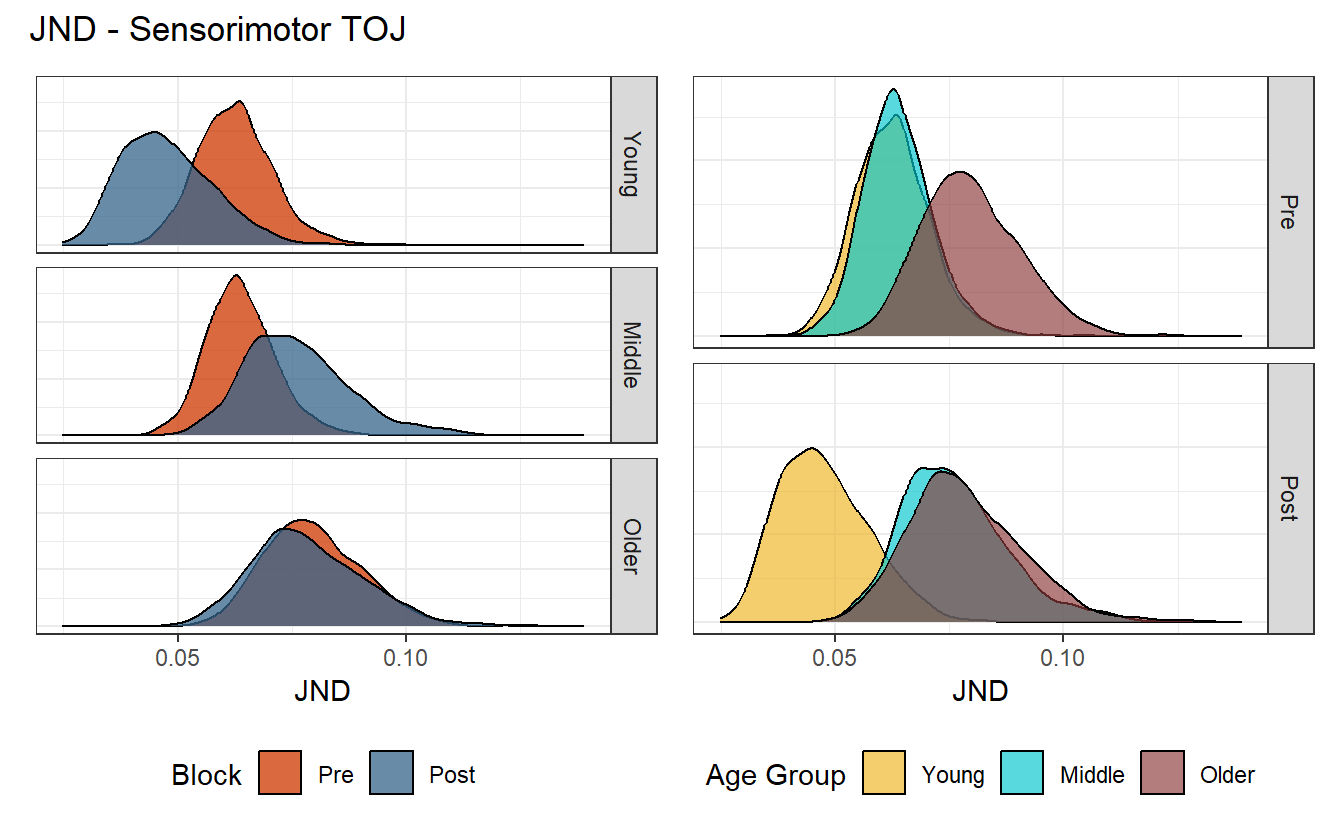
Figure 5.12: Posterior distribution of JND values for the sensorimotor task.
Finally in the sensorimotor task there are mixed results. Temporal recalibration increased the temporal sensitivity in the younger age group, reduced it in the middle age group, and had no effect on the older age group. Clearly the biological factors at play are complex, and the data here is a relatively thin slice of the population. More data and a better calibrated experiment may give better insights into the effects of temporal recalibration.
5.3 Lapse Rate across Age Groups
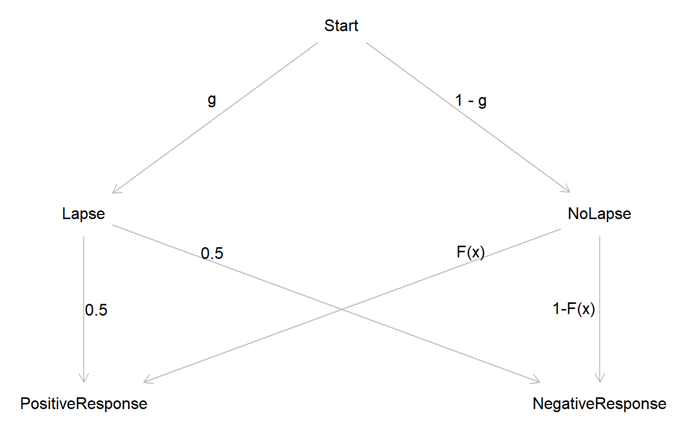
Figure 5.13: Process model of the result of a psychometric experiment with the assumption that lapses occur at random and at a fixed rate, and that the subject guesses randomly in the event of a lapse.
In the above figure, the outcome of one experiment can be represented as a directed acyclic graph (DAG) where at the start of the experiment, the subject either experiences a lapse in judgment with probability \(\gamma\) or they do not experience a lapse in judgment. If there is no lapse, then they will give a positive response with probability \(F(x)\). If there is a lapse in judgment, then it is assumed that they will respond randomly – e.g. a fifty-fifty chance of a positive response. In this model of an experiment, the probability of a positive response is the sum of the two paths.
\[\begin{align*} \mathrm{P}(\textrm{positive}) &= \mathrm{P}(\textrm{lapse}) \cdot \mathrm{P}(\textrm{positive} | \textrm{lapse}) \\ &\quad + \mathrm{P}(\textrm{no lapse}) \cdot \mathrm{P}(\textrm{positive} | \textrm{no lapse}) \\ &= \frac{1}{2} \gamma + (1 - \gamma) \cdot F(x) \end{align*}\]
If we then let \(\gamma = 2\lambda\) then the probability of a positive response becomes
\[ \mathrm{P}(\textrm{positive}) = \lambda + (1 - 2\lambda) \cdot F(x) \]
This is the same lapse model described in (4.15)! But now there is more insight into what the parameter \(\lambda\) is. If \(\gamma\) is the true lapse rate, then \(\lambda\) is half the lapse rate. This may sound strange at first, but remember that equation (4.15) was motivated as a lower and upper bound to the psychometric function where the bounds are constrained by the same amount. Here the motivation is from an illustrative diagram, yet the two lines of reasoning arrive at the same model.
Figure 5.14 shows the distribution of lapse rates for each age group across the four separate tasks. There is no visual trend in the ranks of lapse rates, meaning that no single age group definitively experiences a lower lapse rate than the others, though the middle age group comes close to being the winner and the older age group is more likely to be trailing behind. The distribution of lapse rates does reveal something about the tasks themselves.
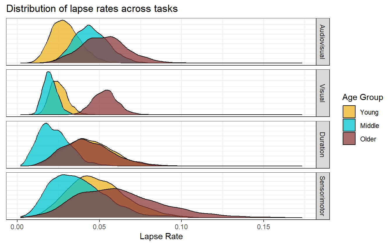
Figure 5.14: Lapse rates for the different age groups across the four separate tasks. Visually there is no clear trend in lapses by age group, but the concentration of the distributions give insight into the perceived difficulty of a task where more diffuse distributions may indiciate more difficult tasks.
We used the audiovisual data in the first few iterations of building a model and there were no immediate issues, but when we tested the model on the visual data it had trouble expressing the variability at outer SOA values. We also noted that one subject had a near perfect response set, and many others had equally impressive performance. The model without a lapse rate was being torn between a very steep slope near the PSS and random variability near the outer SOAs. The remedy was to include a lapse rate (motivated by domain expertise) which allowed for that one extra degree of freedom necessary to reconcile the opposing forces.
Why did the visual data behave this way when the audiovisual data had no issue? That gets deep into the theory of how our brains integrate signals arising from different modalities. Detecting the temporal order of two visual stimuli may be an easier mental task than that of heterogeneous signals. Then consider the audiovisual task versus the duration or sensorimotor task. Visual-speech synthesis is a much more common task throughout the day than visual-tactile (sensorimotor), and so perhaps we are better adjusted to such a task as audiovisual. The latent measure of relative performance or task difficulty might be picked up through the lapse rate.
To test this idea, the TOJ experiment could be repeated, but also ask the subject afterwards how they would rate the difficulty of each task. For now, a post-hoc test can be done by comparing the mean and spread of the lapse rates to a pseudo-difficulty measure as defined by the proportion of the incorrect responses. A response is correct when the sign of the SOA value is concordant with the response, e.g. a positive SOA and the subject gives the “positive” response or a negative SOA and the subject gives the “negative” response. Looking at figure 5.14, we would subjectively rate the tasks from easiest to hardest based on ocular analysis as
- Visual
- Audiovisual
- Duration
- Sensorimotor
Again, this ranking is based on the mean (lower intrinsically meaning easier) and the spread (less diffuse implying more agreement of difficulty between age groups). The visual task has the tightest distribution of lapse rates, and the sensorimotor has the widest spread, so we can rank those first and last respectively. Audiovisual and duration are very similar in mean and spread, but the audiovisual has a bit more agreement between the young and middle age groups, so second and third go to audiovisual and duration. Table 5.1 shows the results arranged by increasing pseudo difficulty. As predicted, the visual task is squarely at the top and the sensorimotor is fully at the bottom. The only out of place group is the audiovisual task for the older age group, which is about equal to the older age group during the duration task. In fact, within tasks, the older age group always comes in last in terms of proportion of correct responses, while the young and middle age groups trade back and forth.
| Task | Age Group | Pseudo Difficulty |
|---|---|---|
| visual | Middle | 0.03 |
| visual | Young | 0.03 |
| visual | Older | 0.06 |
| audiovisual | Young | 0.12 |
| audiovisual | Middle | 0.12 |
| duration | Middle | 0.14 |
| duration | Young | 0.16 |
| duration | Older | 0.17 |
| audiovisual | Older | 0.17 |
| sensorimotor | Young | 0.22 |
| sensorimotor | Middle | 0.24 |
| sensorimotor | Older | 0.29 |
5.4 Subject specific inferences
The multilevel model described by (4.17) provides subject-specific estimation as well as the age group level estimations presented above. If desired, we can make comparisons between subjects or use the subject level estimates to highlight the variation within age groups. Figure 5.15 shows the comparison of two middle aged subjects from the visual TOJ task. They both show heightened temporal sensitivity through an increased slope.
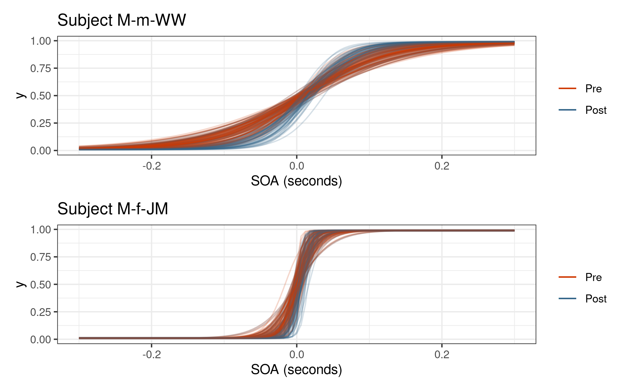
Figure 5.15: Comparison of subject-specific distribution of psychometric functions from the Visual TOJ task.
The subject-level model can make predictions for new individuals or for individuals that did not complete a block. Recall that the post-adaptation block for subject O-f-CE was removed from the audiovisual data set (see figure 3.4). We can still predict their post-adaptation performance because we have information from their pre-adaptation responses and the age-block level estimates as demonstrated in figure 5.16.
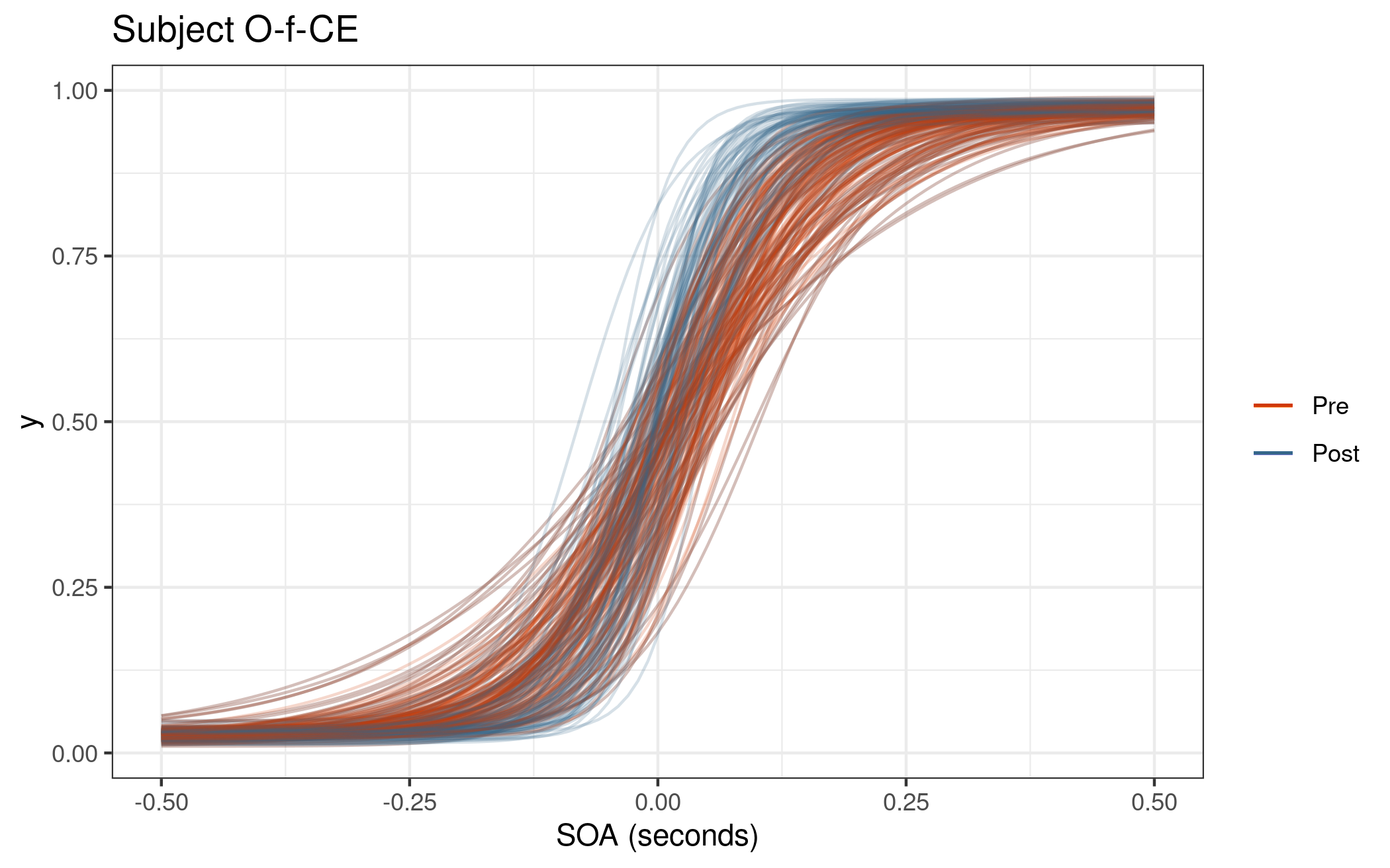
Figure 5.16: Block estimates for subject O-f-CE. Even though their post-adaptation block was not in the data set, we can make predtictions thanks to the multilevel model with subject-level predictors.